Identifiability and parameterization in VAEs

Alex Lee, 2023-01-31

Overall principles of VAEs

Objective: model some random vectors \(\mathbf{x} \in \mathbb{R}^d\) by using a latent variable \(\mathbf{z} \in \mathbb{R}^n\) to structure a deep latent variable model:

\[p_\mathbf{\theta}(\mathbf{x}, \mathbf{z}) = p_\mathbf{\theta}(x \mid\mathbf{z})p_\mathbf{\theta}(\mathbf{z})\]

Where \(\theta \in \Theta\) are parameters of that model.

The model then gives the observed distribution as:

\[p_\theta(x) = \int p_{\mathbf{\theta}}(\mathbf{x}, \mathbf{z}) \mathrm{d}\mathbf{z}\]

What about the data?

We assume there is a data generating process given by:

\(p_{\mathbf{\theta^\ast}}(\mathbf{x}, \mathbf{z}) = p_{\theta^\ast}(\mathbf{x}\mid\mathbf{z}) p_{\theta^\ast}(\mathbf{z}^\ast)\)

with \(\mathbf{\theta}^\ast\) as true but unknown parameters.

We then suppose the processes that generates our data, \(\mathcal{D}\),

\(\mathcal{D} = \{\mathbf{x}^{(1)}, ..., \mathbf{x}^{(\mathit{N})}\}\) is,

\(\mathbf{z}^{\ast(i)} \sim p_{\theta^\ast}(\mathbf{z})\)
\(\mathbf{x}^{(i)} \sim p_{\theta} (\mathbf{x} \mid \mathbf{z}^{\ast(i)})\)

and we optimize using the likelihood such that after optimization:

\(p_{\theta}(\mathbf{x}) \approx p_{\theta^{\ast}}(\mathbf{x})\)

So, what’s the problem? (according to Khemakhem et al.)

In our framework, we learn a generative model: \(p_\theta (\mathbf{x}, \mathbf{z}) = p_\theta (\mathbf{x} \mid \mathbf{z}) p_\theta (\mathbf{z})\) as well as an inference model: \(q_\phi (\mathbf{z} \mid \mathbf{x})\)

The problem is that we generally have no guarantees about what these learned distributions actually are: all we know is that the marginal distribution over \(x\) is meaningful.

Intuitively, we cannot be confident in our inference model \(q_\phi\), because our models are unidentifiable (do not satisfy):

\[\forall(\theta, \theta^{\prime}) : p_\theta(\mathbf{x}) = p_{\theta^\prime} (\mathbf{x}) \implies \theta = \theta^{\prime} \]

and in fact, Locatello (2019) shows ID of disentangled models is impossible for any similar unsupervised model (including \(\beta\)-VAE, TC-VAE, etc.) without inductive bias (or supervision).

Brief aside on the proof of this:

Theorem (Hyvärinen and Pajunen, 1999) Let $ be a d-dimensional random vector of any distribution. Then there exists a transformation \(\mathbf{g}: \mathbf{g}: \mathbb{R}^d \rightarrow \mathbb{R}^d\) such that the components of \(\mathbf{z}^{\prime} := \mathbf{g}(\mathbf{z})\) are independent, and each component has a standardized Gaussian distribution. In particular, \(z_{1}^{\prime}\) equals a monotonic transformation of \(z_1\)

Basically using something like Gram-Schmidt or QR we can always get a new set of variables that are independent and admit Gaussian parameterization. Once we transform it this way, we can take any orthogonal transformation without changing the distribution (something like \(\mathbf{z}^{\prime} = \mathbf{g}^{-1}(M\mathbf{g}(\mathbf{z})\)). As long as the decoder can invert the transformation in this way, we cannot (reliably) recover the true latents based on looking at the data alone.

For further see Appendix of Variational Autoencoders and Nonlinear ICA: A Unifying Framework (Khemakhem, 2020) and I Don’t need u: identifiable non-linear ICA without side information (Willets 2021).

Well, OK, but do we care if VAE models are unidentifiable?

Unfortunately, models are also poor at learning disentangled representations of data (unsupervised)

Here we define disentanglement (informally) as separating the distinct factors of variation, or that a change in a single factor \(z_i\) should lead to a single factor of the representation \(r(\mathbf{x})\).

Or, using a specific approximation called total correlation:
\(C(X_1, ..., X_n) = D_{KL} [p(X_1, ..., X_n)\ ||\ p(X_1)p(X_2) \cdot p(X_n)]\)

The authors (Locatello et al.) train a variety of VAEs (\(\beta\)-VAE, TC-VAE, DIP-VAE, FactorVAE) on a couple of datasets:

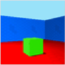
Note that each of these has as “labels” the ground-truth factors of variation.

\(C(X_1, ..., X_n) = D_{KL} [p(X_1, ..., X_n)\ ||\ p(X_1)p(X_2) \cdot p(X_n)]\)

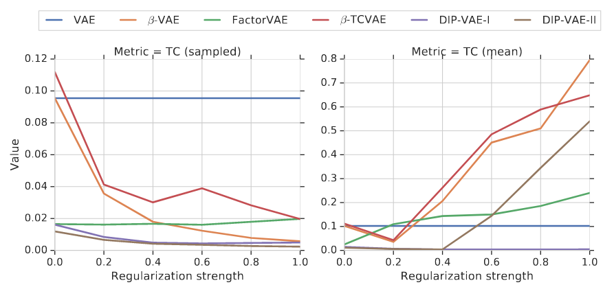
• as regularization goes up (think of \(\beta\)-VAE), \(z\) are disentangled–but only with random sampling
• however, the correlation actually increases when we select the average representation (as we often do)
• disentanglement mildly correlates with downstream accuracy

What is to be done about this?

The authors of Khemakhem (2020) actually show that with supervision, we can have identifiability

We utilize a new variable, \(\mathbf{u}\), to enforce conditional independency of \(\mathbf{z}\) with a new model where:

\[ p_\theta(\mathbf{x}, \mathbf{z}\mid \mathbf{u}) = p_f(\mathbf{x} \mid \mathbf{z}) p_\phi(\mathbf{z} \mid \mathbf{u}) \]

this model forms a Bayes net: \(\mathbf{u} \rightarrow \mathbf{z} \rightarrow \mathbf{x}\) and here, \(\theta\) and \(\phi\) are identifiable up to permutations and scaling–unless \(\mathbf{z}\) are Gaussian with only scale parameters.

The likelihood is: \[ \mathbf{E}_{q_{\phi}(\mathbf{z} \mid \mathbf{x}, \mathbf{u})} [\mathrm{log}\ p_\theta(\mathbf{x}, \mathbf{z} \mid \mathbf{u}) - log_{q_\phi}(\mathbf{z} \mid \mathbf{x}, \mathbf{u})] \]

which can be rewritten: \(\mathrm{log}\ p_\theta(\mathbf{x} \mid \mathbf{u}) - \mathrm{KL}(q_\phi(\mathbf{z} \mid \mathbf{x}, \mathbf{u})\ ||\ p_\theta(\mathbf{z} \mid \mathbf{x}, \mathbf{u}))\)

The salient fact here is that \(\mathbf{u}\) provides the unmixing of \(\mathbf{z}\)

So, then, what is the right variable \(\mathbf{u}\) to condition on, and how should we do it?

There’s a rapidly developing literature in this area, but these two papers present different ideas about this:

Lopez et al. study Perturb-seq analysis with a link to causal learning

The idea is to integrate the idea of sparse mechanism shift:

which says each perturbation only affects a few mechanisms (latents).

The idea is to model this using a sparse a bipartite graph, \(G^a = ([K], [p], E)\), where \(E\) are edges, \([p]\) the number of latents, and \([K]\) denotes the set of perturbations.

note: instead of \(\mathbf{u}\) as the supervising / conditional variable, now we are using \(\mathbf{a}\)

To do this, we modify the normal scVI VAE with a spike-and-slab prior:

\[ z_i\ \mid\ a \sim \gamma_i^a\mathrm{Normal}(\mu_i^a, 1) + (1 - \gamma_i^a)\mathrm{Normal}(0,1),\ \mathbf{z} \in \mathbb{R}^d \\ \pi_i^a \sim \mathrm{Beta}(1, K) \\ \gamma_i^a \sim \mathrm{Bernoulli}(\pi_i^a), \]

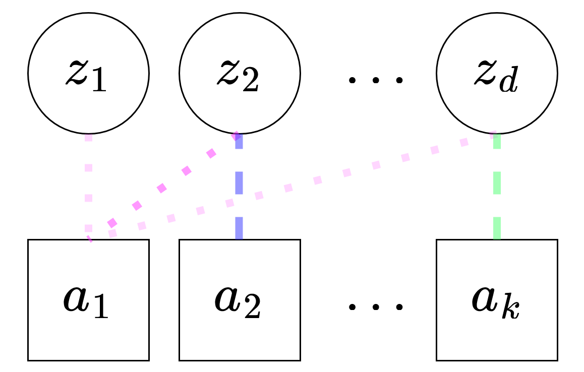
The dotted lines indicate the \(\pi_i^a\)’s learned by the model.

In practice we use a Gumbel-sigmoid to model the Bernoulli.


This formulation gives a identifiability up to linear transformation–stronger than before

This model performs well in simulations of single-cell data

The authors simulate data with this sparse mechanism and try to see if the right \(\pi_i^a\) are learned

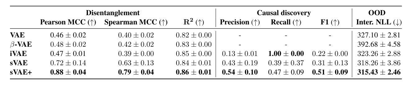
Models were mixed with a small neural network–so I suppose OK that the F1 is quite low-and in general, the iVAE and sVAE were modified in ways that are not exactly correspondent to the original framing to accomodate comparison

Analysis on Replogle (2022) datasets

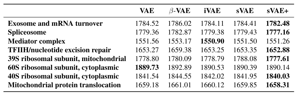
Interventional NLL is highest for sVAE+ on transfer learning task

Hold out sets were defined by manual clustering of perturbations

Conclusions and caveats

• \(\mathrm{Beta}\) distribution may not be coded correctly in the reference implementation (doesn’t seem to incorporate \([K]\))
• Seems like overall model does well at recovering sparse-shift simulated data–does this match biology?
• What are ways to better validate this sort of model? Known gene lists or TF-target lists?
• Logits for \(\pi_i^a\) are scalar values that are optimized; can we use other models / methods to parameterize more flexibly?
• How to interpret \(z\)’s? Paper used post-hoc methods but not LDVAE variants; are there other ways?

Taeb et al. focus on interpretability and predictive accuracy

Assumption: \(\mathbf{z}\) can be partitioned into two parts in to an “anti-causal” model:

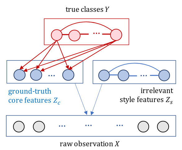
\(\mathbf{z}_c\) and \(\mathbf{z}_s\), where \(s\) denotes “style” features and \(c\) denotes “core” features–only core features are relevant for prediction.

We also set assumptions on the covariance structure of \(\mathbf{z}\)

\[ \mathbf{X} = f^\star(\mathbf{Z}), \mathrm{where}\ \epsilon \perp\kern-5pt\perp \mathbf{Z}, \mathbf{Y} \\ \mathbf{Z}\mid\mathbf{Y} = y \sim \mathcal{N} \Biggl( \begin{pmatrix} \mu_y \\ \mu \end{pmatrix}, \begin{pmatrix} D_y^\star & 0 \\ 0 & G^\star \end{pmatrix} \Biggr),\ D_y^\star\ \mathrm{diagonal} \]

Which basically gives the factorized posterior for \(D_y^\star\) that we are used to and lets the style features have an arbitrary structure.

In this model we also get identifiability up to scaling and permutation (less strong than sVAE+).

This model has a very different architecture, with two portions

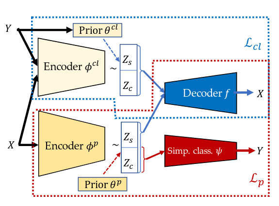
There are two encoders:

• \(\phi_{cl}\), which sees \(\mathbf{Y}\) directly during training
• \(\phi_p\), which only sees \(\mathbf{X}\)

And two decoders:

• \(f\), which actually is used twice every forward pass, once for each set of \(\mathbf{z}\)
• \(\phi\), which simply outputs \(\hat{y}\)

The actual loss then is \(\mathcal{L} = \mathcal{L}_{cl} + \mathcal{L}_{p} - \lambda_n\rho\)

• \(\mathcal{L}_{cl}\) (which is actually two terms, \(f(\phi^p(\mathbf{x}))\) and \(f(\phi^{cl}(\mathbf{x}))\) which helps the \(\mathbf{z}\) converge together and causes “concept learning”
• \(\lambda\rho\) is a group sparsity penalty on the decoder and encoder, separately

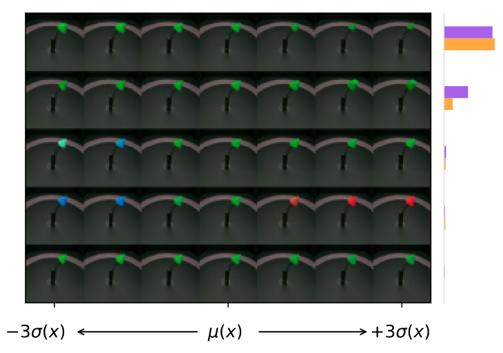
Interpretability is provided in form of latent traversal inspection

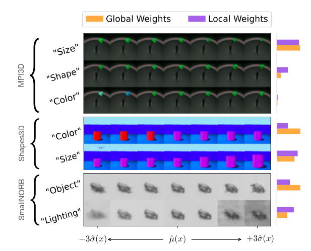
For a given data point, posterior mean is computed and then data points around the source are decoded.

Global vs local weights are from the model or from the data.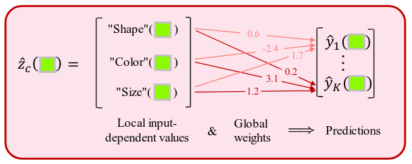

Accuracy is high (>99%) but traversals not incredibly convincing

Regularization is also very important; without \(\lambda\) model seems to be more likely to have low-variance / unimportant dimensions.

In addition, for the datasets shown (Shapes3D and MPI3D) there are many labels–performance and ability to recover meaningful variables decreases with number of labels provided

Exploration on chest x-ray dataset

Dataset has 14 classes; CLAP performs at least as well as comparator model (~90% accuracy)

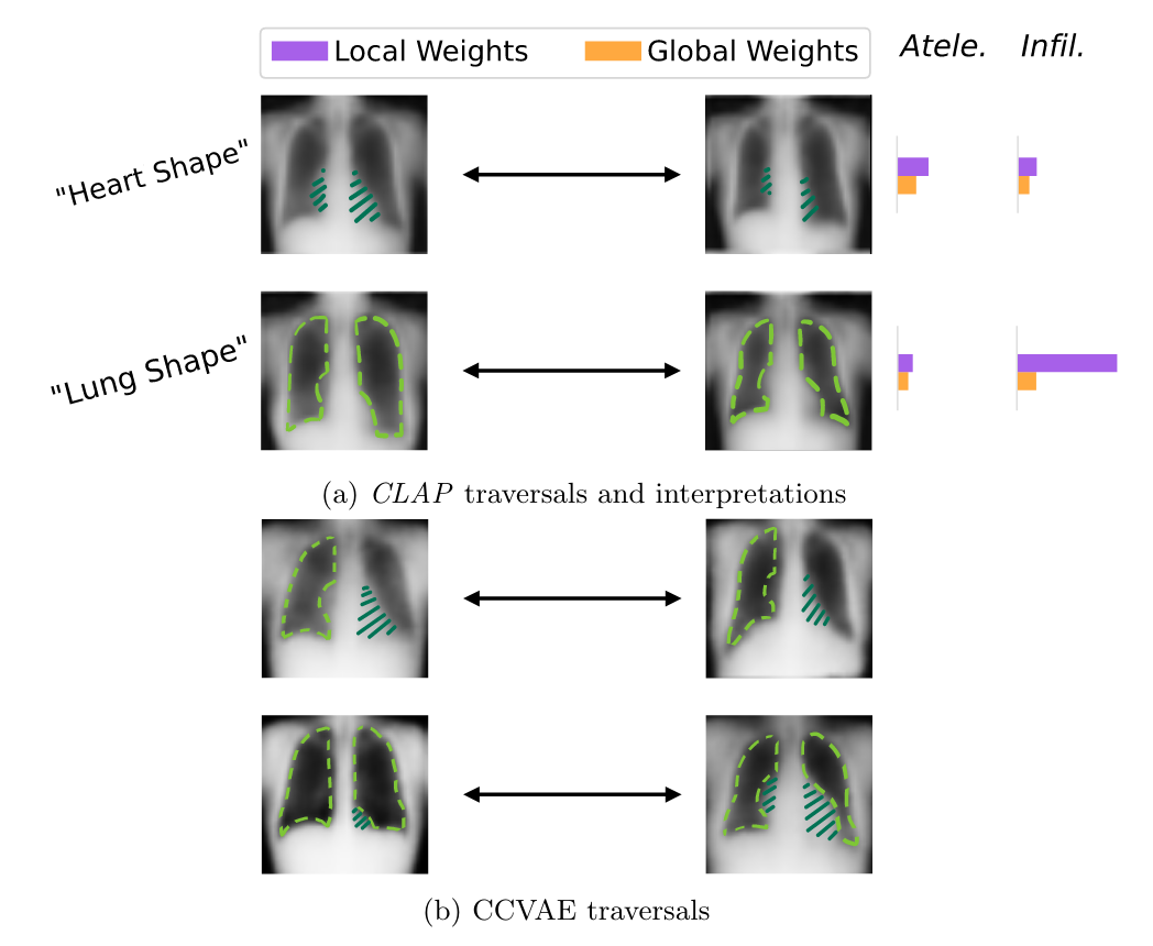
Local vs global weights seem to have some overall relevance for classification (Lung shape feature)

CCVAE does not seem to produce as disentangled features

Authors speculate that low resolution in output images is due to decoder fidelity

Caveats and takeaways

• Relativly simple decoder / prediction architecture
• Unclear how poor performance would be with different types of supervision
• Authors comment various ground-truth features change jointly within traversal – maybe a way in which sVAE+ is probably better
• Would be interesting to use scRNA-seq gene coexpression to interpret \(\mathbf{z}\)
• Not clear if every prediction target has its own \(\phi\) model

Conclusions:

For iVAE, the method focuses on conditional independence of \(\mathbf{u}\) and \(\mathbf{z}\), with no direct parameterization of \(\mathbf{z}\mid\mathbf{x}\)

For sVAE+, focus is on but sparse association of treatments and factors

CLAP the method is much more focused on interpretability, and the anticausal model plays a strong role